Next: Example 4
Up: Numerical examples
Previous: Example 2
In this example we choose another nonlinear partial differential
equation and homogeneous Dirichlet boundary conditions:
This problem has been considered in [16], but without state constraints.
Table 3:
Information on solution of Example 3
| N+1 |
it |
CPU |
Acc |
 |
| 50 |
29 |
131 |
8 |
.110242 |
| 100 |
32 |
2257 |
8 |
.110263 |
| 200 |
31 |
42644 |
8 |
.110269 |
|
Figure 5:
Example 3,
 : Optimal control.
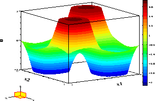 |
Figure 6:
Example 3,
: Optimal state and adjoint variable
 |
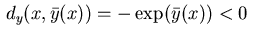
The adjoint equations (2.10), (2.12) yield
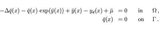 |
(4.4) |
The minimum condition (2.21) leads again to the projection
![\begin{displaymath}
\bar{u}(x) = P_{\,[u_1,u_2]}\,(\bar{q}(x)/\alpha)
\end{displaymath}](img164.gif) |
(4.5) |
with
![$\,[u_1,u_2] = [-5,5]\,$](img165.gif) .
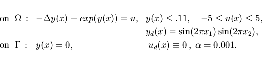
The optimal control is shown in Figure 5, while Figure 6 displays the
optimal state and associated adjoint variable.
The adjoint variable allows to verify the control rule (4.5).
Note that condition (2.7) does not hold for this example
in view of
.
The optimal control is shown in Figure 5, while Figure 6 displays the
optimal state and associated adjoint variable.
The adjoint variable allows to verify the control rule (4.5).
Note that condition (2.7) does not hold for this example
in view of
 .
.
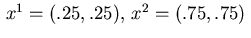
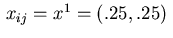
The state is active in the points
 .
In view of the decomposition (2.15), the measure
.
In view of the decomposition (2.15), the measure  is
given here by the singular measure
is
given here by the singular measure
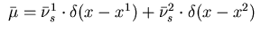 , where
 are identified with the multipliers
  in view of
(3.15). Let us check now the accuracy with which the computed
adjoint equation is satisfied. At the point
in view of
(3.15). Let us check now the accuracy with which the computed
adjoint equation is satisfied. At the point
 we obtain
 .
Then the discretized adjoint equation (3.11) yields
.
Then the discretized adjoint equation (3.11) yields
 for
for  .
.
Next: Example 4
Up: Numerical examples
Previous: Example 2
Hans D. Mittelmann
2000-10-06