

Next: Example 2
Up: Numerical examples
Previous: Numerical examples
In this example we choose a nonlinear partial differential
equation and homogeneous Dirichlet boundary conditions:
These equations are related to a simplified Ginzburg-Landau model
for super-con- ductivity in the absence of internal magnetic fields
with  the wave function;
cf. Ito, Kunisch [19] and Kunisch, Volkwein [20].
The adjoint equations (2.10), (2.12) apply:
 |
(4.1) |
Since  , the minimum condition (2.21) yields the
control law
![\begin{displaymath}
\bar{u}(x) = P_{\,[u_1,u_2]}\,(\bar{q}(x)/\alpha) \,,
\end{displaymath}](img146.gif) |
(4.2) |
where
![$\,P_{\,[u_1,u_2]}\,$](img147.gif) denotes the projection operator onto the interval
denotes the projection operator onto the interval
![$\,[u_1,u_2] = [1.5,4.5]\,$](img148.gif) .
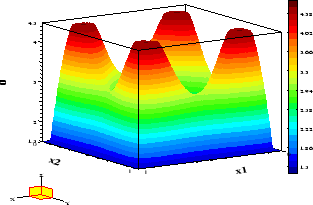
The optimal control is shown in Figure 1, while Figure 2 depicts the
optimal state and associated adjoint variable.
The adjoint variable permits the verification of
the control law (4.2).
The state is active in the center
.
The optimal control is shown in Figure 1, while Figure 2 depicts the
optimal state and associated adjoint variable.
The adjoint variable permits the verification of
the control law (4.2).
The state is active in the center  .
Figure 2 indicates that condition (2.7) is not satisfied since
 holds for all
  .
However, well-posedness of the Ginzburg-Landau model follows from
results in Gunzburger et al. [15].
Figure 1:
Example 1
 : Optimal control.
 |
Figure 2:
Example 1,
 : Optimal state and adjoint variable
 |
Table 1:
Information on solution of Example 1
| N+1 |
it |
CPU |
Acc |
 |
| 50 |
26 |
104 |
8 |
.0577903 |
| 100 |
30 |
1897 |
8 |
.0621615 |
| 200 |
35 |
54831 |
8 |
.0644259 |
|
Figure 3:
Example 2,  : Optimal control and switching curve
 .
.
 |
Figure 4:
Example 2,  : Optimal state and adjoint variable
 |


Next: Example 2
Up: Numerical examples
Previous: Numerical examples
Hans D. Mittelmann
2000-10-06


![]() the wave function;
cf. Ito, Kunisch [19] and Kunisch, Volkwein [20].
the wave function;
cf. Ito, Kunisch [19] and Kunisch, Volkwein [20].