A boundary control example

In this section an example from heat conduction is chosen to demonstrate the viability of the proposed approach. It is meant to be typical for practical problems that have to be solved in industrial and other applications. A mathematical description of the problem is as follows. The underlying boundary value problem is Laplace's equation on the unit square, corresponding to no internal heat sources, coupled with mixed boundary conditions, namely homogeneous Neumann conditions on $x_2 = 0$, or no heat flux across this boundary, a heat flux proportional to the temperature at the boundaries $x_1 = 0$ and $x_1 = 1$, while the solution is controlled on $x_2 = 1$. The control function is to be found such that the temperature in the central subsquare of length $\,0.5\,$ is as close as possible to a given function $y_d = 1$ in the $L_2$-norm. In the first version of the problem a multiple $\,\alpha\,$ of a regularizing boundary integral over the control function is added to the objective functional, while without this a bang-bang control may be expected in the second version. To complete the problem definition upper and lower bounds of $10$ respectively $0$ are imposed on both state and control.

Thus letting $\,\Gamma_2 =\{\,(x_1,1) \, \vert \; 0 \leq x_1 \leq 1 \,\}\,$ and $\,\Omega_0= [0.25,0.75]^2 \,$, the control problem is to determine a function $\,u \in L^{\infty}(\Gamma_2) \,$ which minimizes

$$F(y,u) = \frac{1}{2} \int_{\Omega_0} (y(x)-1)^2\,dx \,+\, \frac{\alpha}{2}\, \int_{\Gamma_2} u(x)^2\,dx$$ (1)

subject to the state equation, Neumann and Dirichlet boundary conditions and control and state inequality constraints,

$$\begin{array}{rlllll} - \Delta y(x) &=& 0 \hspace*{20mm} &... ...q& 10 & \mbox{for} & x_2=1, & 0 \leq x_1 \leq 1 \,. \end{array}$$ (2)

The NLP-problem to be solved is given by (3)-(9). It is a linearly constrained convex quadratic program.

Case $\,\alpha > 0 \,$: The following table lists the results for four different optimization packages with an AMPL interface and one, BPMPD, which was applied after translating the AMPL file into extended MPS format. For a reference to AMPL, the codes, and the MPS format as well as for other benchmarks, see [31]. An asterisk denotes failure, while otherwise the CPU seconds on a Linux-PC with 450MHz PII and 512 MB are listed. The optimization problem of the largest instance has $32,757$ variables and $32,578$ constraints. A probable reason for the failures of SNOPT and MINOS is the near linear independence of the equality constraints which causes an increasing ill-conditioning with growing N.

Table 1: Results for Example 4.1, $\alpha = 0.005$

N	LOQO	SNOPT	LANC	MINOS	BPMPD	$F$
60	13	41	1126	18	4	.2789728
120	203	*	29561	369	*	.2590819
180	722	*	*	*	186	.2530543

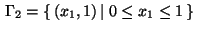
Figure 1: Example 4.1, $\alpha = 0.005$ : Optimal control on $\,\Gamma _2$ and adjoint variable $q_{iN}$ .

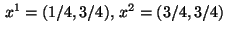
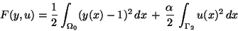
Figure 2: Example 4.1, $\,\alpha = 0.005$ : Optimal state and adjoint variable on $\,\Omega \,$.

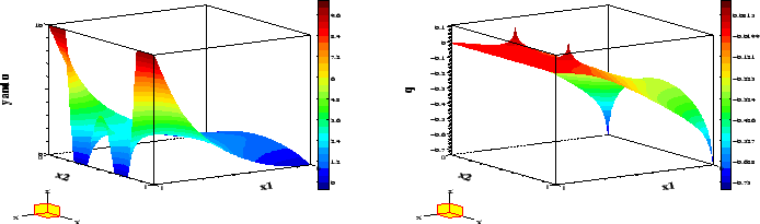The optimal control and adjoint variable for the weight $\,\alpha=0.005\,$ are shown in Figure 1. It is instructive to discuss the necessary conditions (19)-(23) that apply in this case. The state constraint $\,y(x) \leq 3.15\,$ for $\,x \in \Omega_0\,$ becomes active at two points $\,x^1 =(1/4,3/4),\,x^2 = (3/4,3/4)\,$, while the state constraint $\,y(x) \leq 10\,$ in $\,\Omega \setminus \Omega_0\,$ does not become active. Hence, the adjoint equations (19) are

$$\hspace*{-10mm} \begin{array}{rlll} -\Delta \bar{q}(x) + \ba... ...) & = 0 & \quad \mbox{on} & \;\; \Gamma_2 \,, \quad \end{array}$$ (3)

where the measure is given by $\,\bar{\mu}= \bar{\nu}^1_s\,\delta(x-x^1) + \bar{\nu}^2_s\,\delta(x-x^2)\,$ . The approximation (15) yields the values $\, \bar{\nu}^1_s = \bar{\nu}^2_s =-0.198746 \,$. The optimal state and adjoint variable on $\,\Omega \,$ are displayed in Figure 2.

The minimum condition reduces to the case (22) with $\,x \in \Gamma_2\,$ since no control is applied on the Neumann boundary $\,\Gamma_1\,$. In view of $\,u_d(x) = 0 \,$ we get from (22) for all $\,x=(x_1,1), \,0 \leq x_1 \leq 1\,$:

$$\hspace*{-9mm} \bar{u}(x) = \left \{ \begin{array}{llllll} ... ...l_{\nu}\bar{q}(x)/\alpha \,\geq 10\,, \end{array}\right \} \;$$ (4)

In order to evaluate its discrete analogon, we recall definition (5) and relation (17) which give

$$\partial_{\nu}\bar{q}(x_{i,N+1}) \, \sim \, -q_{iN} / h \,, \quad i=1,...,N \,.$$

Hence, the discrete version of the minimum condition (4) requires to check the conditions

$$\hspace*{-9mm} u_{i,N+1} = \left \{ \begin{array}{llllll} q... ...pha*h) \;\geq 10 \end{array}\right \} \,, \; i = 1,...,N \, .$$ (5)

By inspecting Figure 1, the reader may verify this condition for the value $\,\alpha=0.005\,$.

Case $\,\alpha=0\,$: Table 2 lists the results for the five optimization packages used in Table 1.

Table 2: Results for Example 4.1, $\,\alpha = 0$

N	LOQO	SNOPT	LANC	MINOS	BPMPD	$F$
60	15	149	1516	17	5	.1771073
120	220	*	25868	398	57	.1574154
180	939	*	*	*	243	.1512835

Figure 3: Example 4.1, $\,\alpha = 0$ : Optimal state and control.

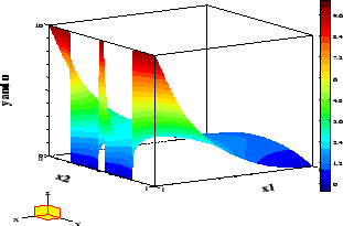Figure 4: Example 4.1, $\,\alpha = 0$ : Optimal control on $\,\Gamma _2\,$ and switching function $\,q_{iN}\,$ .

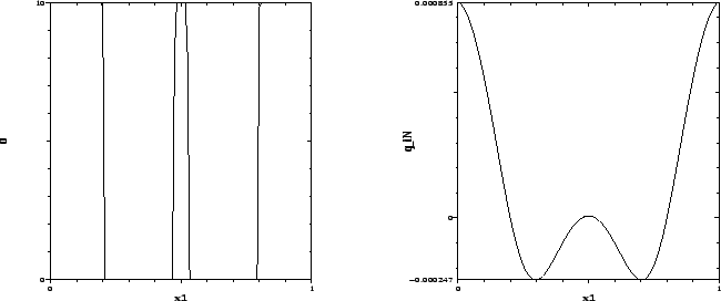Figure 5: Example 4.1, $\,\alpha = 0$ : Adjoint variable on $\,\Omega \,$.

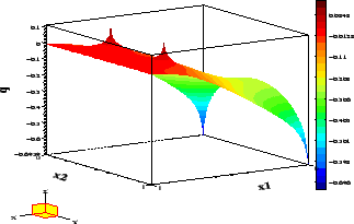The adjoint equation agrees with equation (3). The optimal control shown in Figure 4 is bang-bang. Accordingly, the minimum condition (24) yields the control law

$$\hspace*{-8mm} \bar{u}(x) = \left \{ \begin{array}{llllll} u... ...;\; \partial_{\nu}\bar{q}(x) < 0 \\ \end{array}\right \} \, .$$ (6)

Its discrete variant yields in analogy to (5),

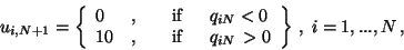$$\hspace*{-9mm} u_{i,N+1} = \left \{ \begin{array}{llllll} 0... ...;\; q_{iN} \,> 0 \end{array}\right \} \,, \; i = 1,...,N \, ,$$ (7)

which is confirmed by Figure 4.