Next: Distributed Control Problem
Up: Necessary conditions for elliptic
Previous: Necessary conditions for elliptic
We consider the problem of determining a boundary control function
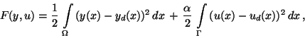
 which minimizes the functional
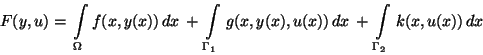 |
(1) |
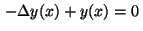
subject to the elliptic state equation,
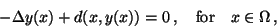 |
(2) |
boundary conditions of Neumann or Dirichlet type,
and control and state inequality constraints,
| |
|
 |
(5) |
| |
|
 |
(6) |
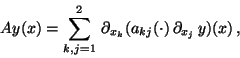
The functions
 and
and
 are assumed to be
  -functions.
It is straightforward to include more than one inequality constraint in (5) or (6).
However, since both the state and control variable are scalar variables,
the active sets for different inequality constraints are disjoint and
hence can be treated separately.
-functions.
It is straightforward to include more than one inequality constraint in (5) or (6).
However, since both the state and control variable are scalar variables,
the active sets for different inequality constraints are disjoint and
hence can be treated separately.
The Laplacian  in (2)
can be replaced by any elliptic operator
in (2)
can be replaced by any elliptic operator
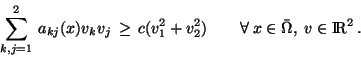
where the coefficients
 satisfy the
following coercivity condition with some
satisfy the
following coercivity condition with some  :
:
However, in the sequel we restrict the discussion to the operator
 which simplifies the form of the necessary conditions
and the numerical analysis.
which simplifies the form of the necessary conditions
and the numerical analysis.
An optimal solution of problem (1)-(6) will be
denoted by  and
and  .
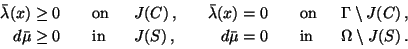
The active sets for the inequality constraints
(5), (6) are defined by
.
The active sets for the inequality constraints
(5), (6) are defined by
 |
(7) |
The following regularity conditions are supposed to hold,
 |
(8) |
Here and in the following, partial derivatives are denoted by subscripts.
First order necessary conditions for the rather general problem
(1)-(6) are not yet available in the literature.
The main difficulty results from the Dirichlet condition (4)
which prevents solution from being sufficiently regular.
First order necessary conditions for problems with linear elliptic
equations
 and pure Neumann conditions
may be found in Casas [14], Casas et al. [15,16].
A weak formulation for linear elliptic equations and Dirichlet conditions
is due to Bergounioux, Kunisch [4].
and pure Neumann conditions
may be found in Casas [14], Casas et al. [15,16].
A weak formulation for linear elliptic equations and Dirichlet conditions
is due to Bergounioux, Kunisch [4].
We shall present first order conditions in a form that can
be derived at least in a purely formal way. This form will turn out to be
consistent with the first order conditions of Kuhn-Tucker for the discretized elliptic control problem in section 3.1.
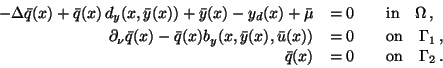
We assume that there exists an
adjoint state
 ,
a multiplier
,
a multiplier
 ,
and a regular Borel measure
,
and a regular Borel measure  on
on  such that the following conditions hold:
adjoint equation and boundary conditions:
minimum condition for
 :
:
 |
(12) |
minimum condition for
 :
:
 |
(13) |
complementarity conditions:
 |
(14) |
The adjoint equations (9)-(11) are understood
in the weak sense, cf. Casas et al. [16].
According to Bourbaki [10], Chapter 9, the regular Borel measure
appearing in the adjoint equation (9)
has the decomposition
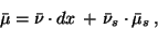 |
(15) |
where  represents the Lebesgue measure and
 is singular
with respect to ; the functions
is singular
with respect to ; the functions
 are
measurable on .
The problem of obtaining the decomposition (15) explicitly
is related to the difficulty of determining the structure of the active set
are
measurable on .
The problem of obtaining the decomposition (15) explicitly
is related to the difficulty of determining the structure of the active set
 .
In section 3, we shall make an attempt to approximate the measure by the
multipliers of the discretized control problem.
.
In section 3, we shall make an attempt to approximate the measure by the
multipliers of the discretized control problem.
In many applications, the cost functional (1) is of
tracking type, cf. [2,4,22,24],
 |
(16) |
with given functions
 ,
and nonnegative weight
,
and nonnegative weight
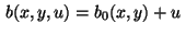
 The control and state constraints (5) and (6)
are taken to be box constraints of the simple type
The control and state constraints (5) and (6)
are taken to be box constraints of the simple type
 |
(17) |
with functions
 and
and
 .
Here, in particular we assume that the functions
.
Here, in particular we assume that the functions  and
and  in (1) coincide.
For these data the adjoint equations (9)-(11) become
in (1) coincide.
For these data the adjoint equations (9)-(11) become
 |
(18) |
If the function  in the Neumann condition (3)
has the special form
in the Neumann condition (3)
has the special form
 ,
then the minimum condition (12) reduces to
,
then the minimum condition (12) reduces to
![\begin{displaymath}
\hspace*{-8mm}
[\alpha (\bar{u}(x)-u_d(x)) - \bar{q}(x)] \, ...
...uad \forall \, x \in \Gamma_1, \; u \in [u_1(x),u_2(x)] \,. \;
\end{displaymath}](img74.gif) |
(19) |
Likewise, if the function  in (4)
is given by
in (4)
is given by
 ,
the minimum condition (13) yields
,
the minimum condition (13) yields
![\begin{displaymath}
\hspace*{-7mm}
[\alpha (\bar{u}(x)-u_d(x)) + \partial_{\nu} ...
...uad \forall \, x \in \Gamma_2, \; u \in [u_1(x),u_2(x)] \,. \;
\end{displaymath}](img77.gif) |
(20) |
Case
 : The previous conditions determine the following
control laws:
: The previous conditions determine the following
control laws:
for
,
 |
(21) |
for
,
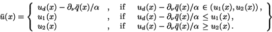 |
(22) |
Case  : We obtain an optimal control of
bang-bang or singular type:
: We obtain an optimal control of
bang-bang or singular type:
for
,
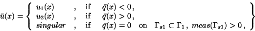 |
(23) |
for
,
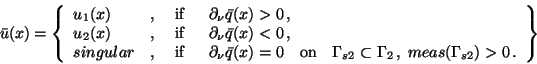 |
(24) |
Hence in case , the so-called switching function is
given by the adjoint function
 on the boundary
 resp. by
the outward normal derivative
resp. by
the outward normal derivative
 on the boundary
  .
The isolated zeros of the switching function are the switching points
of a bang-bang control; cf. the example in section 4.1.
.
The isolated zeros of the switching function are the switching points
of a bang-bang control; cf. the example in section 4.1.
Next: Distributed Control Problem
Up: Necessary conditions for elliptic
Previous: Necessary conditions for elliptic
Hans D. Mittelmann
2000-12-09