A distributed control example

In this section we consider an optimal control problem for a semilinear elliptic equation of logistic type which was studied in Leung, Stojanovic [25,34]. The problem is to determine a distributed control $\, u \in L^{\infty}(\Omega)\,$ that minimizes the functional

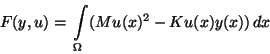$$F(y,u) = \, \int \limits_{\Omega} (Mu(x)^2 - Ku(x)y(x))\,dx \, \quad$$ (8)

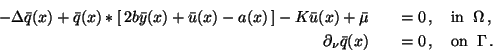
subject to the elliptic state equation

$$-\Delta y(x) = y(x)(a(x)-u(x)-by(x)) \,, \quad \mbox{for} \quad x \in \Omega \,,$$ (9)

homogeneous Neumann boundary conditions,

$$\hspace*{17mm} \partial_{\nu} y(x) = 0 \,, \quad \mbox{for} \quad x \in \Gamma\,,$$ (10)

and control and state inequality constraints

$$u_1 \leq u(x) \leq u_2 \quad y(x) \leq \psi(x)\,, \quad \mbox{for} \quad x \in \Omega \,.$$ (11)

Here, $y(x)$ denotes the population of a biological species, $a(x)$ a spatially dependent intrinsic growth rate, $b$ the crowding effect, while $F$ denotes the difference between economic cost and revenue, with nonnegative constants $\,M, K\,$. The goal is to find a control function which maximizes profit. A similar control problem with Dirichlet boundary conditions was recently studied by Cañada et al. [12]. Three numerical methods, two of interior point type, were compared in [2] for linear problems and homogeneous Dirichlet conditions.

The adjoint equations (33), (34) applied to problem (8)-(11) lead to

$$\begin{eqnarray*} -\Delta \bar{q}(x) + \bar{q}(x)*[\,2 b \bar{y}(x) + \bar{u}(x... ...partial_{\nu}\bar{q}(x) &&=0 \,, \quad \mbox{on} \;\; \Gamma \,. \end{eqnarray*}$$

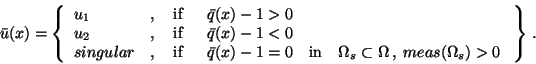
The minimum condition (40) gives the following two control laws. For
$\,M > 0\,$ we get

$$\bar{u}(x) = P_{[u_1,u_2]} \left ( \frac{1}{2M}\,[\,(K - \bar{q}(x))\,\bar{y}(x)\,] \right ) \,,$$ (12)

where $\,P_{[u_1,u_2]}\,$ denotes the projection operator on the interval $\,[u_1,u_2]\,$. In case $\,M=0\,$ we can put $\,K=1\,$ and obtain

$$\hspace*{-8mm} \bar{u}(x) = \left \{ \begin{array}{llllll} u... ...mega \,, \; meas(\Omega_s) > 0 \; \end{array}\right \} \,. \;$$ (13)

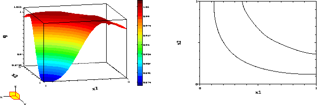
Figure 6: Optimal control and state for Example 4.2, $M = 1, K=0.8$ .

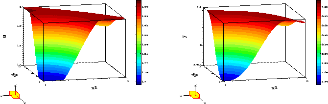For the sake of reference the data were chosen as in [25], Example 5.2:

$$a(x) = 7 + 4 \sin(2\pi x_1 x_2), \;b = 1, \;M=1, \;K=0.8 \,.$$

For this case the computational approach of [25] is not valid. Additionally, bound and state constraints were chosen: $\,u_1 = 1.7$, $u_2 = 2$, $\psi(x) = 7.1$. Both types of bounds become active. The optimal control and state are shown in Figure 6. The reader may verify that the control law (12) is satisfied. The state variable attains its upper bound at the two points $\,x^1=(0.21,0.99),\,x^2=(0.99,0.21)\,$ near the boundary. It has to be noted that this example leads to a difficult nonlinear optimization problem which is not a QP anymore but a quadratically constrained quadratic program. Thus, the QP solver BPMPD is not applicable. For testing the local optimality of the computed solution, second-order sufficient conditions would need to be evaluated. To the best of our knowledge for this class of elliptic problems the literature does not provide a verifiable set of such conditions. A practical test could be devised by checking the positive definiteness of the projected Hessian of the Lagrangian. This test will be part of our future work.

In the following tables an asterisk denotes failure and an "m" that the available memory was exceeded. The fact that made the previous problem and those in [28,29] difficult for SQP-based methods, namely the near linear dependence of the constraints, here the discretized boundary value problem, which exhibits increasing ill-conditioning for growing $N$, is even more pronounced through the homogeneous Neumann conditions resulting in singular constraints. The largest instance has $79,998$ variables and $40,397$ constraints in the NLP problem. These results were obtained on a HP9000-K260 with 256MB.

Table 3: Results for Example 4.2, $\,M=1, K=0.8$ .

N	LOQO	SNOPT	LANC	MINOS	$F$
50	218	3281	2356	289	-6.485781
100	2141	m	103794	5331	-6.576428
200	28517	m	*	*	-6.620092

Table 4: Results for Example 4.2, $\,M=0, K=1$ .

N	LOQO	SNOPT	LANC	MINOS	$F$
50	77	7384	3704	267	-18.48254
100	3012	m	116328	*	-18.73615
200	57264	m	*	*	-18.86331

To confirm that a bang-bang control can occur in this problem the case $\,M = 0$, $K = 1$, $u_1 = 2$, $u_2 = 6$, $\psi(x) = 4.8$ was solved. The optimal control and state are shown in Figure 7. Both the control and the state constraints become active. The adjoint variable and the switching curves $\bar q(x) = 1$ displayed in Figure 8 admit a verification of the control law (13). While the CPU times for $N = 200$ are excessive, the accuracy for $N=100$ should be sufficient and the times are acceptable. To avoid the trivial solution $y = 0$ of the state equation nonzero starting values for the state were chosen in this example. As in the case $M = 1$, the local optimality of the solution shown in Figure 7 would need to be verified.

Figure 7: Optimal control and state for Example 4.2, $M = 0, K = 1$.

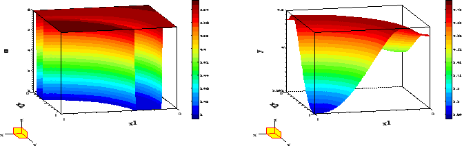Figure 8: Optimal adjoint variable and switching curves for Example 4.2, $M = 0, K = 1$.