Management Problem

In this section, we will look at the following model [2]:

$$\begin{array}{rcl} \mbox{min } & \sum_{i=1}^nc_i+d_ix_i+\frac... ... \quad i=1:n,\\ & x_i: \mbox{integer},\quad i=1:n. \end{array}$$ (3-1)

This model can be interpreted as a multi-item production and inventory management problem with a limited resource, where the $x_i$ are called decision variables [17,20]. In general, the objective function minimizes the cost, which could be the sum of setup (ordering) costs, inventory holding costs, and purchase costs. The constraints provide the restrictions of a shared resource as well as non-shared resources. Moreover, the model represents numerous application problems based on the interpretations of the decision variables. There are at least four different applications using the model (3-1).

Let us consider the continuous relaxation of (3-1). In order to solve it as a second-order cone problem, we must ensure that (3-1) can be cast as SOCP. Let $t=$max$_j \frac{1}{x_j}$. Then $tx_j\geq 1,$ for all $j$. We introduce a $s$ in this inequality and rewrite it as

$$\begin{array}{rcl} tx_j&\geq& s^2, \quad \mbox{ for all } j\\ \mbox{with }s &=& 1. \end{array}$$

By using the following fact [5]:

$$\omega^2 \leq xy,\quad x\geq 0,\quad y\geq 0 \Longleftrightarrow \left\Vert\begin{pmatrix}2\omega\cr x-y\end{pmatrix}\right\Vert \leq x+y,$$ (3-2)

the previous inequality becomes

$$\left \Vert \begin{pmatrix}2\cr t-x_j\end{pmatrix}\right\Vert \leq t+x_j,$$    for all $$j.$$

Therefore, we can rewrite the inequalities as

$$2^2+(t-x_j)^2 \leq (t+x_j)^2,$$    for all $$j.$$

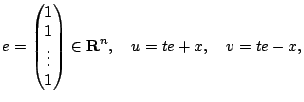
Next, define $e$, $u$,$v$, and $w$ as follows,

$$e=\begin{pmatrix}1\cr 1\cr \vdots\cr 1\end{pmatrix}\in{\bf R}^n,\quad u=te+x,\quad v=te-x,$$ and $$w=2e.$$

It is then clear that $x=\frac{u-v}{2}$ and $te=\frac{u+v}{2}$. Plugging this into our model, we obtain

$$\begin{array}{rcl} \mbox{min}& \sum_{i=1}^n c_i+d_i(\frac{u-v... ...uad i=1:n,\\ & u_i^2 \geq v_i^2+w_i^2,\quad i=1:n. \end{array}$$ (3-3)

In this form, the objective function and constraints, except the last $n$ inequalities, are linear. Therefore, we can rewrite them as LP. Each of the last $n$ constraints is a quadratic cone with $u_i$, $v_i$, and $w_i$. We use the random problems described in [2] to generate test cases.

Example 1. Given $50\leq n \leq 200$, $S_i\in [5,20]$, $H_i\in [1,4]$, $D_i\in [10,100]$, $T_i\in [1,15]$, $l_i, u_i \in [8,25]$, $i=1,\cdots,n.$ The total machine time available $T_t$ is generated to ensure the feasibility of problems, i.e.,

$$T_t=\sum_{i=1}^nT_i\bar{x}_i+$$random positive number$$,$$

where $l_i\leq \bar{x}_i\leq u_i,$ for all $i.$ In Chapter 5, we use Example 1 with $n=50,75,100,200$ as part of our testing set.