Next: Long-step path-following method
Up: Numerical realization and results
Previous: Numerical realization and results
Here, we will discuss some computational issues in second order
cone programming, especially the linear system
(1-6). Denote by
![$ [r_1,r_2,r_3,r_4,r_5]^T$](img325.gif) the right
hand side of (1-6). The augmented system following
from (1-6) is
where
the right
hand side of (1-6). The augmented system following
from (1-6) is
where
 We use the NT
direction, i.e.,
We use the NT
direction, i.e.,
 , apply the
Sherman-Morrison-Woodury formula to the coefficient matrix, and
denote
, apply the
Sherman-Morrison-Woodury formula to the coefficient matrix, and
denote
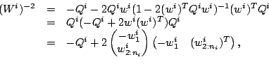
 |
(4-1) |
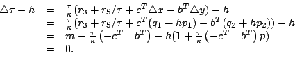
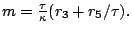
Hence,
 where where 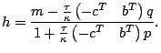 |
(4-2) |
The next lemma follows immediately.
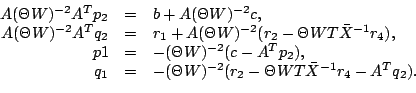
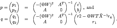
Moreover, the normal equations are
Subsequently,
the search direction can be computed as follows:
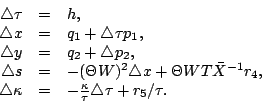
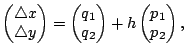
Furthermore, one can rewrite
 as
Two vectors
as
Two vectors
 and
and  have been calculated
while computing
have been calculated
while computing  and
and  Because of the definition of
 ,
,  and
and
 are easy to obtain:
since
are easy to obtain:
since
Next: Long-step path-following method
Up: Numerical realization and results
Previous: Numerical realization and results
Hans D. Mittelmann
2003-09-10