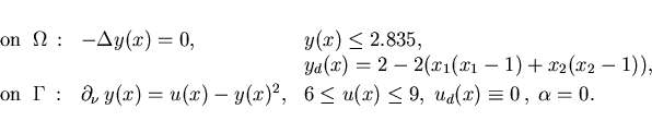
Example 5.5: The first problem has a linear partial differential equation and nonlinear Neumann boundary conditions with data:
Cost functional :
![]() , CPU seconds : 494
, CPU seconds : 494
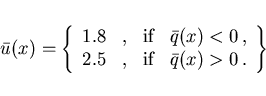
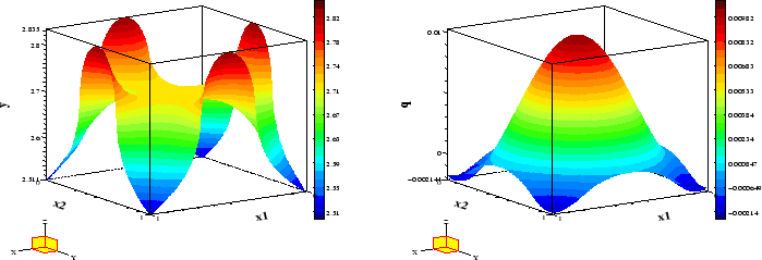
The optimal control and state are shown in Figures 8 and 9.
Note that the sign condition (2.5) holds since
![]() .
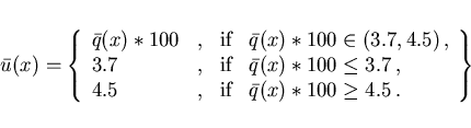
The optimal control is continuous and has
two boundary arcs with
.
The optimal control is continuous and has
two boundary arcs with
![]() and one boundary arc with
and one boundary arc with
![]() . The junction points with the boundary are the
points
. The junction points with the boundary are the
points
![]() on the bottom edge of
on the bottom edge of ![]() .
The control law (2.16) was derived under the assumption
.
The control law (2.16) was derived under the assumption
![]() which obviously holds in this example.
By looking at the adjoint variable in Figure 8, the reader may verify
that the control law (2.16) is satisfied:
which obviously holds in this example.
By looking at the adjoint variable in Figure 8, the reader may verify
that the control law (2.16) is satisfied:
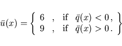
Example 5.6: The data for the second Neumann problem are:
According to the optimal control law (2.17) we can expect either a bang-bang or a singular control. We get the following results:
Cost functional :
![]() , CPU seconds : 864
, CPU seconds : 864
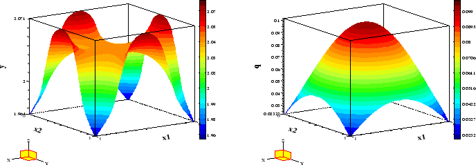
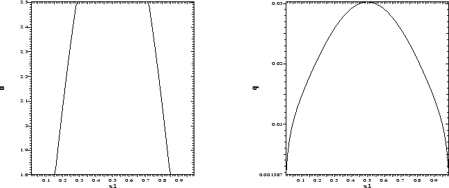
The optimal control in Figure 10 is indeed bang-bang.
The switching function ![]() on
on ![]() as shown in Figure 10
obeys the optimal control law (2.17):
as shown in Figure 10
obeys the optimal control law (2.17):
Example 5.7: In this example we choose a nonlinear partial differential equation and linear Neumann boundary conditions:
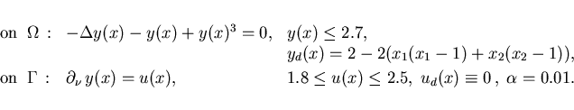
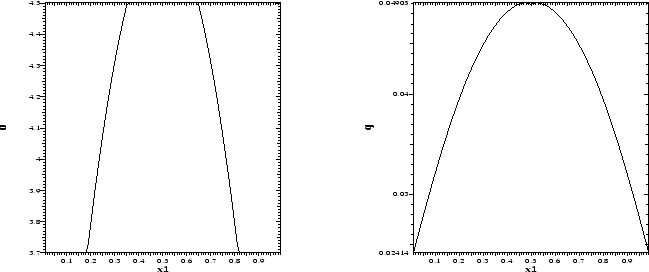
These equations represent a simplified Ginzburg-Landau model
for super-conductivity in the absence of internal magnetic fields
with ![]() the wave function;
cf. Ito, Kunisch [16] and Kunisch, Volkwein [18]
where tracking functions and control or state constraints
have been considered that are different from those used here.
LOQO and AMPL provide the results:
the wave function;
cf. Ito, Kunisch [16] and Kunisch, Volkwein [18]
where tracking functions and control or state constraints
have been considered that are different from those used here.
LOQO and AMPL provide the results:
Cost functional :
![]() , CPU seconds : 317
, CPU seconds : 317
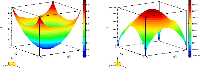
The optimal control and state are shown in Figures 12 and 13.
The optimal control is continuous and has
two boundary arcs with
![]() and one boundary arc with
and one boundary arc with
![]() . The junction points with the boundary are the
points
. The junction points with the boundary are the
points
![]() on the bottom edge of
on the bottom edge of ![]() .
The adjoint variable in Figure 12 shows that
the control law (2.16) is satisfied:
.
The adjoint variable in Figure 12 shows that
the control law (2.16) is satisfied:

Example 5.8:
The data are those from Example 5.7 but now we choose
![]() expecting to obtain a bang-bang control.
The numerical results are:
expecting to obtain a bang-bang control.
The numerical results are:
Cost functional :
![]() , CPU seconds : 570
, CPU seconds : 570
The optimal control shown in Figure 14 is indeed bang-bang.
The switching function ![]() on
on ![]() as shown in Figure 14
yields the optimal control law (2.17):
as shown in Figure 14
yields the optimal control law (2.17):