Computer simulations

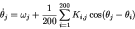
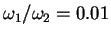
We performed numerical simulations of these models using the method of lines. In this, we model the integrodifferential equation using a set of 200 ordinary differential equations. In the cases presented here, the connection polarities are taken to be $\psi\equiv 0$, the components of f and of K are cosines, and we solved the system

$$\dot\theta_j=\omega_j+\frac{1}{200} \sum_{i=1}^{200}K_{i,j}\cos(\theta_j-\theta_i)$$

for $j=1,\cdots,200$.

A series of computations was done for the single and double layer cases. In the two examples presented here, the initial data had the form

$$\theta_j(0)=j2\pi/200+R_j$$

for $j=1,\cdots,200$, where R_j is a uniformly distributed random variable having $\vert R_j\vert\le 2\pi/10$.

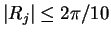We calculate the solutions to time $t=1000\pi$using an adaptive step Runge-Kutta scheme of orders 7 and 8 [12], and by that time the solution had achieved the form $\theta\approx s+c t$and the wave speed (c) is estimated by evaluating $\theta_1(1000\pi)/1000\pi$.

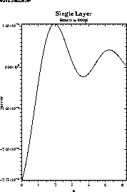
The results of the single layer simulation are shown in the Figure 1. In this, $\omega = 1, N=1,L=\pi$and the predicted wave speed is $1+\pi$. In Figure 2 we plot the numerical error, which is deviation of our calculated solution from the theoretical solution derived above

$$\left\vert 1-\frac{\theta_{computed}(s,T)-\theta(0,T)}{s}\right\vert$$

at $T=1000 \pi$. We see there that the error is O(10^-6)for this simulation.

  

Figure: Initial data (top) and calculated solution $\theta _j(1000\pi )$ (bottom). In this case, $c_{obs}\approx 4.14$ and $c_{calc}=1+\pi$.

  

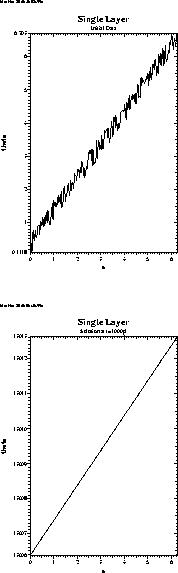Figure 2: Error of our computer simulation of the single layer model shown in Figure 1.

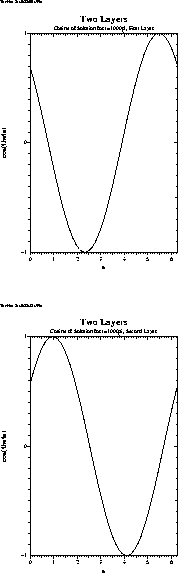
In the case of two layers, we take similar initial data for each of the two layers as described above, but we take $\omega_1/\omega_2=0.01$. The results are shown in Figure 3 This simulation demonstrates that a striated structure can support different wave speeds.

  

Figure: Plotted here are $\cos\theta_{1,j}(1000\pi)$ (top) and $\cos\theta_{2,j}$ (bottom). The estimated wave speeds in these cases are c₁ = 5.01 and c₂ =0.264.