Example 6, an elliptic system of logistic type

In this section we consider an optimal control problem for a semilinear elliptic equation of logistic type which was studied in Leung, Stojanovic [21,28]. The problem is to determine a distributed control $\, u \in L^{\infty}(\Omega)\,$ that minimizes the functional

$$F(y,u) = \, \int \limits_{\Omega} (Mu(x)^2 - Ku(x)y(x))\,dx \, \quad$$ (4.7)

subject to the elliptic state equation

$$-\Delta y(x) = y(x)(a(x)-u(x)-by(x)) \,, \quad \mbox{for} \quad x \in \Omega \,,$$ (4.8)

homogeneous Neumann boundary conditions,

$$\partial_{\nu} y(x) + \beta(x) y(x)= 0 \,, \quad \mbox{for} \quad x \in \Gamma\,,$$ (4.9)

and control and state inequality constraints

$$u_1 \leq u(x) \leq u_2 \quad y(x) \leq \psi(x)\,, \quad \mbox{for} \quad x \in \Omega \,.$$ (4.10)

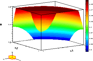
Figure 11: Example 6 : Optimal control.

Figure 12: Example 6 : Optimal state and adjoint variable

Here, $y(x)$ denotes the population of a biological species, $a(x)$ a spatially dependent intrinsic growth rate, $b$ the crowding effect, while $F$ denotes the difference between economic cost and revenue, with nonnegative constants $\,M, K\,$. In [21,28] the function $\,\beta(x)\,$ was chosen as $0$. Numerical results for this case can be found in [25]. Here, we consider $\,\beta(x) = 1\,$ if $x_1 = 0$ or $x_2 = 0$ and $\,\beta(x) = 0\,$ otherwise. The goal is to find a control function which maximizes profit. A similar control problem with Dirichlet boundary conditions was recently studied by Cañada et al. [8].

The adjoint equations (2.10), (2.11) yield the following equations:

$$\begin{eqnarray*} -\Delta \bar{q}(x) + \bar{q}(x) [\,2 b\,\bar{y}(x) + \bar{u}(... ...}(x) + \beta(x) \bar{q}(x) = 0 \,, && \mbox{on} \;\; \Gamma \,. \end{eqnarray*}$$

For $\,M > 0\,$, the minimum condition (2.18) gives the control law

$$\bar{u}(x) = P_{\,[u_1,u_2]} \left ( \frac{1}{2M}\,[\,(K - \bar{q}(x))\,\bar{y}(x)\,] \right ) \,,$$ (4.11)

where $\,P_{\,[u_1,u_2]}\,$ denotes the projection operator on the interval $\,[u_1,u_2]\,$.

The following concrete data were used:

$$\begin{array}{l} a(x) = 7 + 4 \sin(2\pi x_1 x_2),\,b = 1,\,M... ...=0.8, \\ [1mm] u_1=1.4,\,u_2=1.6, \,\psi(x)=6.09\,. \end{array}$$

Figure 11 displays the optimal control while Figure 12 shows the optimal state and adjoint variable. The reader may verify that the minimum condition given by the projection (4.11) holds with high accuracy. However, note that condition (2.7) imposed in [6] is not satisfied everywhere in $\Omega$.

Table 7: Information on solution of Example 6

N+1	it	CPU	Acc	$F(\bar{y})$
50	29	104	8	-4.19322
100	32	2235	8	-4.27569
200	33	42543	8	-4.31709